(Iterative) Hirshfeld method
In this tutorial, we will introduce how to use the horton_part API method to execute (iterative) Hirshfeld partitioning methods.
First, we import the required libraries.
[1]:
import logging

import numpy as np
from gbasis.evals.eval import evaluate_basis
from gbasis.wrappers import from_iodata
from grid import AtomGrid, ExpRTransform, UniformInteger
from iodata import load_one
from setup import prepare_grid_and_dens, print_results

from horton_part import HirshfeldIWPart, HirshfeldWPart, ProAtomDB, ProAtomRecord
from horton_part.scripts.generate_cube import (
    _setup_cube_grid,
    prepare_input_cube,
    to_cube,
)

np.set_printoptions(precision=3, linewidth=np.inf, suppress=True)
In (iterative) Hirshfeld methods, a database of atomic radial density profiles is required. Therefore, different single-atom DFT or other ab initio calculations should be executed. Here, we use the Gaussian package. The checkpoint files, in fchk format, are generated using Gaussian tools as well.
Next, the radial atomic density is obtained by computing the spherical average of the atomic density. This process can be applied using the gbasis and grid packages.
[2]:
def prepare_record(filename):
    """Prepare molecular grid and density."""
    mol = load_one(filename)

    # Specify the integration grid
    rtf = ExpRTransform(5e-4, 2e1, 120 - 1)
    uniform_grid = UniformInteger(120)
    rgrid = rtf.transform_1d_grid(uniform_grid)

    # Get the spin-summed density matrix
    one_rdm = mol.one_rdms.get("post_scf", mol.one_rdms.get("scf"))
    basis = from_iodata(mol)
    assert len(mol.atnums) == 1
    grid = AtomGrid.from_preset(atnum=mol.atnums[0], preset="fine", rgrid=rgrid)

    basis_grid = evaluate_basis(basis, grid.points)
    rho = np.einsum("ab,bp,ap->p", one_rdm, basis_grid, basis_grid, optimize=True)
    spline = grid.spherical_average(rho)
    radial_rho = spline(rgrid.points)

    record = ProAtomRecord(mol.atnums[0], mol.charge, mol.energy, rgrid, radial_rho)
    return record
In this tutorial, we focus on the water molecule and therefore only need data for hydrogen and oxygen atoms. It should be noted that data for both cations and anions are also used.
[3]:
h_1 = prepare_record("./data/atoms/001__h_001_q+00/mult02/atom.fchk")
h_2 = prepare_record("./data/atoms/001__h_002_q-01/mult01/atom.fchk")
o_7 = prepare_record("./data/atoms/008__o_007_q+01/mult04/atom.fchk")
o_8 = prepare_record("./data/atoms/008__o_008_q+00/mult03/atom.fchk")
o_9 = prepare_record("./data/atoms/008__o_009_q-01/mult02/atom.fchk")

records = [h_1, h_2, o_7, o_8, o_9]
db = ProAtomDB(records)
Next, we prepare the molecular grid and densities as described in the Basic Usage section. It should be noted that the radial grids for atoms in the water molecule should match the atomic radial grids used for the corresponding single atoms in the atomic database calculations.
[4]:
def prepare_argument_dict(mol, grid, rho, db):
    """Prepare basic input arguments for all AIM methods."""
    kwargs = {
        "coordinates": mol.atcoords,
        "numbers": np.asarray(mol.atnums, np.int64),
        "pseudo_numbers": mol.atnums,
        "grid": grid,
        "moldens": rho,
        "lmax": 3,
        "proatomdb": db,
    }
    return kwargs
Hirshfeld method
The Hirshfeld method can be executed using the HirshfeldWPart class.
[5]:
mol, grid, rho = prepare_grid_and_dens("data/h2o.fchk")
h = HirshfeldWPart(**prepare_argument_dict(mol, grid, rho, db))
h.do_all()
print_results(h)
The number of electrons: 10.000003764139395
Coordinates of the atoms
 [[ 0.     0.     0.224]
 [-0.     1.457 -0.896]
 [-0.    -1.457 -0.896]]
Atomic numbers of the atom
 [8 1 1]

================================================================================
Information of integral grids.
--------------------------------------------------------------------------------
Grid size of molecular grid: 18460
************************************ Atom 0 ************************************
   |-- Radial grid size: 120
   |-- Angular grid sizes:
          6 6 6 6 6 6 6 6 6 6 6 6 6 6 6 6 6 6 6 6
          6 6 6 6 6 6 6 6 6 6 6 6 6 6 6 6 6 6 6 6
          6 6 6 18 18 18 18 18 18 18 18 18 18 18 18 18 18 18 18 18
          18 18 18 18 18 18 26 26 26 26 38 38 38 38 38 50 50 50 50 50
          86 86 110 110 110 110 170 194 194 434 590 590 434 434 434 302 302 302 194 194
          170 110 110 110 110 110 110 110 110 110 110 110 86 50 50 18 18 18 18 18

************************************ Atom 1 ************************************
   |-- Radial grid size: 120
   |-- Angular grid sizes:
          6 6 6 6 6 6 6 6 6 6 6 6 6 6 6 6 6 6 6 6
          6 6 6 6 6 6 6 6 6 6 6 6 6 6 6 6 6 6 6 6
          6 6 6 6 6 6 6 6 6 6 6 6 6 6 6 18 18 18 18 18
          18 18 18 18 18 18 18 18 18 26 26 26 38 38 38 38 38 38 38 50
          50 50 50 50 50 86 86 86 110 110 110 170 170 170 194 194 194 194 170 170
          170 110 110 110 110 110 110 110 110 110 110 86 86 50 50 50 18 18 18 18

************************************ Atom 2 ************************************
   |-- Radial grid size: 120
   |-- Angular grid sizes:
          6 6 6 6 6 6 6 6 6 6 6 6 6 6 6 6 6 6 6 6
          6 6 6 6 6 6 6 6 6 6 6 6 6 6 6 6 6 6 6 6
          6 6 6 6 6 6 6 6 6 6 6 6 6 6 6 18 18 18 18 18
          18 18 18 18 18 18 18 18 18 26 26 26 38 38 38 38 38 38 38 50
          50 50 50 50 50 86 86 86 110 110 110 170 170 170 194 194 194 194 170 170
          170 110 110 110 110 110 110 110 110 110 110 86 86 50 50 50 18 18 18 18

--------------------------------------------------------------------------------
================================================================================

Performing a density-based AIM analysis with a wavefunction as input.
  Molecular grid    : MolGrid
  Using local grids : True
Initialized: HirshfeldWPart
  Scheme       : Hirshfeld
  Proatomic DB : <horton_part.core.proatomdb.ProAtomDB object at 0x104443c10>
Computing atomic populations.
Computing atomic charges.
Computing density decomposition for atom 0
Computing density decomposition for atom 1
Computing density decomposition for atom 2
Computing cartesian and pure AIM multipoles and radial AIM moments.
Computing atomic dispersion coefficients.
Storing proatom density spline for atom 0.
Storing proatom density spline for atom 1.
Storing proatom density spline for atom 2.
charges:
[-0.305  0.153  0.153]
cartesian multipoles:
[[-0.305 -0.    -0.    -0.253 -4.416 -0.    -0.    -3.647 -0.    -4.093 -0.    -0.    -0.637 -0.    -0.    -0.    -0.    -0.247 -0.    -1.401]
 [ 0.153 -0.     0.167 -0.131 -0.758 -0.    -0.    -0.643  0.035 -0.689 -0.     0.206 -0.2   -0.    -0.    -0.     0.468 -0.127  0.164 -0.454]
 [ 0.153  0.    -0.167 -0.131 -0.758  0.     0.    -0.643 -0.035 -0.689 -0.    -0.206 -0.2   -0.    -0.    -0.    -0.468 -0.127 -0.164 -0.454]]
Iterative Hirshfeld method
The iterative Hirshfeld method can be executed using HirshfeldIWpart class.
[6]:
hi = HirshfeldIWPart(**prepare_argument_dict(mol, grid, rho, db))
hi.do_all()
print_results(hi)
================================================================================
Information of integral grids.
--------------------------------------------------------------------------------
Grid size of molecular grid: 18460
************************************ Atom 0 ************************************
   |-- Radial grid size: 120
   |-- Angular grid sizes:
          6 6 6 6 6 6 6 6 6 6 6 6 6 6 6 6 6 6 6 6
          6 6 6 6 6 6 6 6 6 6 6 6 6 6 6 6 6 6 6 6
          6 6 6 18 18 18 18 18 18 18 18 18 18 18 18 18 18 18 18 18
          18 18 18 18 18 18 26 26 26 26 38 38 38 38 38 50 50 50 50 50
          86 86 110 110 110 110 170 194 194 434 590 590 434 434 434 302 302 302 194 194
          170 110 110 110 110 110 110 110 110 110 110 110 86 50 50 18 18 18 18 18

************************************ Atom 1 ************************************
   |-- Radial grid size: 120
   |-- Angular grid sizes:
          6 6 6 6 6 6 6 6 6 6 6 6 6 6 6 6 6 6 6 6
          6 6 6 6 6 6 6 6 6 6 6 6 6 6 6 6 6 6 6 6
          6 6 6 6 6 6 6 6 6 6 6 6 6 6 6 18 18 18 18 18
          18 18 18 18 18 18 18 18 18 26 26 26 38 38 38 38 38 38 38 50
          50 50 50 50 50 86 86 86 110 110 110 170 170 170 194 194 194 194 170 170
          170 110 110 110 110 110 110 110 110 110 110 86 86 50 50 50 18 18 18 18

************************************ Atom 2 ************************************
   |-- Radial grid size: 120
   |-- Angular grid sizes:
          6 6 6 6 6 6 6 6 6 6 6 6 6 6 6 6 6 6 6 6
          6 6 6 6 6 6 6 6 6 6 6 6 6 6 6 6 6 6 6 6
          6 6 6 6 6 6 6 6 6 6 6 6 6 6 6 18 18 18 18 18
          18 18 18 18 18 18 18 18 18 26 26 26 38 38 38 38 38 38 38 50
          50 50 50 50 50 86 86 86 110 110 110 170 170 170 194 194 194 194 170 170
          170 110 110 110 110 110 110 110 110 110 110 86 86 50 50 50 18 18 18 18

--------------------------------------------------------------------------------
================================================================================

Performing a density-based AIM analysis with a wavefunction as input.
  Molecular grid    : MolGrid
  Using local grids : True
Initialized: HirshfeldIWPart
  Scheme                : Hirshfeld-I
  Convergence threshold : 1.0e-06
  Maximum iterations    : 500
  Proatomic DB          : <horton_part.core.proatomdb.ProAtomDB object at 0x104443c10>
Iteration       Change      Entropy
        1   4.91894e-02   2.00489e-01
        2   3.09349e-02   1.80862e-01
        3   1.95877e-02   1.90830e-01
        4   1.26979e-02   2.03872e-01
        5   8.40308e-03   2.14964e-01
        6   5.64913e-03   2.23432e-01
        7   3.84155e-03   2.29631e-01
        8   2.63387e-03   2.34078e-01
        9   1.81637e-03   2.37237e-01
       10   1.25775e-03   2.39468e-01
       11   8.73435e-04   2.41038e-01
       12   6.07777e-04   2.42140e-01
       13   4.23518e-04   2.42912e-01
       14   2.95413e-04   2.43453e-01
       15   2.06199e-04   2.43832e-01
       16   1.43998e-04   2.44098e-01
       17   1.00594e-04   2.44283e-01
       18   7.02895e-05   2.44413e-01
       19   4.91226e-05   2.44503e-01
       20   3.43338e-05   2.44567e-01
       21   2.39993e-05   2.44611e-01
       22   1.67764e-05   2.44642e-01
       23   1.17278e-05   2.44664e-01
       24   8.19875e-06   2.44679e-01
       25   5.73174e-06   2.44690e-01
       26   4.00710e-06   2.44697e-01
       27   2.80143e-06   2.44702e-01
       28   1.95853e-06   2.44706e-01
       29   1.36925e-06   2.44709e-01
       30   9.57279e-07   2.44710e-01

Computing atomic populations.
Computing atomic charges.
Computing density decomposition for atom 0
Computing density decomposition for atom 1
Computing density decomposition for atom 2
Computing cartesian and pure AIM multipoles and radial AIM moments.
Computing atomic dispersion coefficients.
Storing proatom density spline for atom 0.
Storing proatom density spline for atom 1.
Storing proatom density spline for atom 2.
charges:
[-0.862  0.431  0.431]
cartesian multipoles:
[[-0.862  0.    -0.     0.189 -5.147 -0.    -0.    -4.812 -0.    -5.012 -0.    -0.    -0.105  0.     0.     0.     0.     0.58  -0.     0.174]
 [ 0.431 -0.     0.077 -0.04  -0.392 -0.    -0.    -0.389  0.02  -0.375 -0.     0.088 -0.057  0.     0.    -0.     0.264 -0.039  0.083 -0.136]
 [ 0.431  0.    -0.077 -0.04  -0.392  0.     0.    -0.389 -0.02  -0.375  0.    -0.088 -0.057  0.    -0.     0.    -0.264 -0.039 -0.083 -0.136]]
Export AIM density to a cube file
First, a new cube grid must be constructed and the molecular density evaluated at the grid points. Next, the AIM density is recalculated on this cube grid using the AIM weight functions obtained from the partitioning method (e.g., h or hi).
[7]:
def update_pro(part, iatom, proatmdens, grid):
    """Update propars.

    Parameters
    ----------
    iatom : int
        The index of the atom for which the pro-atom densities are to be updated.
    proatdens : 1D np.ndarray
        The array representing the pro-atom density. This array is updated with the new density values
        for the specified atom.
    grid : Grid
        A `Grid` object, e.g., Molecular grid or a 3D cubic grid.
    """
    work = np.zeros((grid.size,))
    part.eval_proatom(iatom, work, grid)
    proatmdens += work
    proatmdens += 1e-100


def compute_aimdens(part, grid, moldens):
    """See ``Compute AIM density.

    Parameters
    ----------
    part : HirshfeldWPart or HirshfeldIWPart.
        A partitioning method.
    grid : Grid
        A `Grid` object, e.g., Molecular grid or a 3D cubic grid.
    moldens : 1D np.ndarray
        Molecular density on `grid` points.
    """
    proatmdens = np.zeros((part.natom, grid.size))
    for iatom in range(part.natom):
        update_pro(part, iatom, proatmdens[iatom, :], grid)
    promoldens = np.sum(proatmdens, axis=0)

    at_weights = np.zeros((part.natom, grid.size))
    # Compute the atomic weights by taking the ratios: pro-atom-dens/pro-molecule-dens.
    for iatom in range(part.natom):
        at_weights[iatom, :] = proatmdens[iatom, :] / promoldens
    np.clip(at_weights, 0, 1, out=at_weights)
    aimdens = at_weights * moldens[None, :]
    return proatmdens, promoldens, at_weights, aimdens
[8]:
logger = logging.getLogger("__main__")
# A denser grid points should be applied to reproduce correct population.
cube_grid = _setup_cube_grid(mol.atnums, mol.atcoords, logger, spacing=0.2)
cube_grid, data = prepare_input_cube(mol, 1000, False, False, logger, cube_grid)
cube_moldens = data["density"]
proatmdens, promoldens, at_weights, aimdens = compute_aimdens(
    hi, cube_grid, cube_moldens
)

sum_pop = 0.0
for iatom in range(hi.natom):
    pop = cube_grid.integrate(aimdens[iatom, :])
    print(f"The population of atom {iatom} using cube_grid is : {pop:.3f}")
    sum_pop += pop
    # export AIM density of each atom in water to a cube file
    to_cube(
        f"h2o_aimrho_{iatom}.cube",
        mol.atnums,
        mol.atcorenums,
        mol.atcoords,
        cube_grid,
        aimdens[iatom, :],
    )
    # export pro-atom density to a cube file
    to_cube(
        f"h2o_prorho_{iatom}.cube",
        mol.atnums,
        mol.atcorenums,
        mol.atcoords,
        cube_grid,
        proatmdens[iatom, :],
    )

# Note: the pupulation of sum of all atoms is not equal to 10 due to a coarse cube grid used.
print(f"The total population using cube_grid is : {sum_pop:.3f}")
print(
    f"The total population using partitioning grid is : {hi.grid.integrate(hi._moldens):.3f}"
)
# export molecular density of water to cube file
to_cube(
    "h2o_molrho.cube",
    mol.atnums,
    mol.atcorenums,
    mol.atcoords,
    cube_grid,
    cube_moldens,
)
# export pro-molecular density of water to cube file
to_cube(
    "h2o_promolrho.cube",
    mol.atnums,
    mol.atcorenums,
    mol.atcoords,
    cube_grid,
    cube_moldens,
)
The population of atom 0 using cube_grid is : 8.404
The population of atom 1 using cube_grid is : 0.540
The population of atom 2 using cube_grid is : 0.540
The total population using cube_grid is : 9.484
The total population using partitioning grid is : 10.000
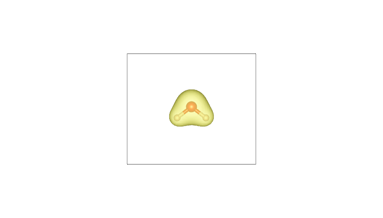
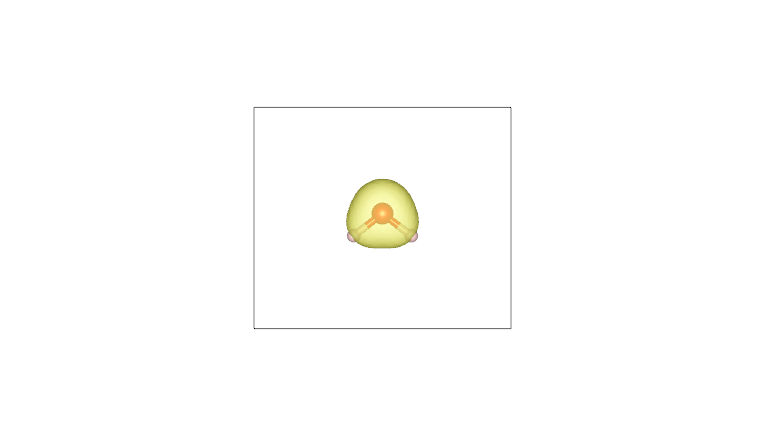
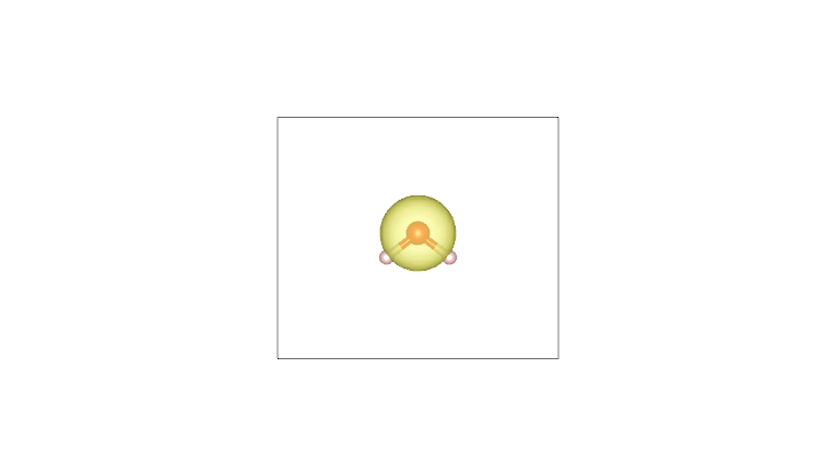
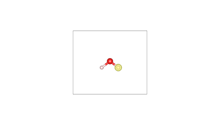
By plotting these cube files with a visualization program such as VESTA (using an isosurface value of 0.05), one obtains the following:
|
|
|---|---|
Molecular density |
Pro-molecular density |

|
|
|---|---|
AIM density (O) |
Pro-atom density (O) |
|
|
|---|---|
AIM density (H) |
Pro-atom density (H) |

[9]:
import glob

# remvoe all cube files
import os

for f in glob.glob("*.cube"):
    os.remove(f)
[ ]: